To gain a better understanding of the current state of education in Fair Haven, I started by building a data set. This document shares the process I went through to combine state and federal resources to generate data sets that would enable an analysis of student outcomes, educational inputs, and their relationship over time. The process also includes a discussion of how I created a set of suitable comparison school districts for Fair Haven.
In an effort to be as transparent as possible, this document contains descriptions of source and derived data sets as well as code in the R programming language that one can use to reproduce results.
Code - Load libraries
options(width =120)library(tidyverse)library(readxl)library(googlesheets4)library(googledrive)library(haven)library(cluster)library(MASS)library(ggpmisc)library(ggrepel)library(ggfortify)library(glue)library(DT)library(htmltools)library(factoextra)library(gt)library(purrr)set.seed(2024)# Commonly used State ID numbers (staid) and Federal Local Education Authority (LEA) IDs# for FH, Little Silver, Rumson, and Shrewsburyfh_leaid <-"3404950"fh_staid <-"NJ-251440"ls_leaid <-"3408790"ls_staid <-"NJ-252720"rums_leaid <-"3414370"rums_staid <-"NJ-254570"shrews_leaid <-"3414970"shrews_staid <-"NJ-254770"district_name_colors <-c("Fair Haven Boro"="#4169E1","Little Silver Boro"="#1F2868","Rumson Boro"="#8640C4","Shrewsbury Boro"="#004500","Other"="darkgrey")
Common Core of Data
The first data set I leverage is the Common Core of Data, a directory of PK-12 schools curated by the Federal Government. The most recent data is specific to the 2023-24 school year, which is suitable for the purpose of building a directory of public, non-charter NJ districts that that offer grades PK/K-8 like Fair Haven.
I identify 267 public, non-charter NJ districts that that offer grades PK/K-8 like Fair Haven. These are saved as a CSV file for easy access.
Click to show/hide table of districts
ACS EDGE
ACS EDGE, or the American Community Survey (ACS) Education Demographic and Geographic Estimates (EDGE), data contains district-level social, economic, housing, and demographic detail based on the ACS 5-year summary files. I use this data to generate peer districts (comparison groups) for Fair Haven. The latest available data was the 2018-22 data, and I use the Population Group: Total Population. The raw data that was downloaded from ACS came as zipped XLSX files. The zip files were uploaded to a Google Drive folder, where they could be accessed and parsed. The collapsed code chunk below creates data frames from the raw ACS EDGE data.
Code - Read ACS EDGE Files from Google Drive
#Auth Google Drive and Sheetsdrive_auth(path ="../pmcrosta-datascience-ed9fcc88faf6.json")gs4_auth(path ="../pmcrosta-datascience-ed9fcc88faf6.json")edge_zips <-drive_find(pattern='edge', type='zip') %>% dplyr::select(name, id)## download, unzip, and clean up files. create edge_* data frames.obnames <-vector()for (ii in1:nrow(edge_zips)) { temp <-tempfile(fileext =".zip") dl <-drive_download(as_id(edge_zips$id[ii]), path = temp, overwrite =TRUE) out <-unzip(temp, exdir =tempdir()) outtxt <-grep(pattern="txt$", x = out, value = T) object_name <-str_remove(edge_zips$name[ii], ".zip")assign(object_name, read.table(outtxt, sep="|", header=T) %>% dplyr::select(-ends_with("moe"))) outxls <-grep(pattern="xlsx$", x = out, value = T) data_dict <-read_excel(outxls, sheet="DP_TotalPop") %>% dplyr::filter(varname %in%colnames(get(object_name))) newnames <- data_dict$varnamenames(newnames) <- data_dict$vlabel duplicate_cols <-duplicated(as.list(get(object_name))) df_unique <-get(object_name)[!duplicate_cols] newnames <- newnames[newnames %in%colnames(df_unique)]assign(object_name, df_unique %>% dplyr::rename(all_of(newnames))) obnames <-c(obnames, object_name)}glue("Data frames created: ", paste(obnames, collapse=", "))
Created `edge_df`. `edge_df` has 557 rows and 44 columns.
edge_df now has the following columns and definitions:
Identifiers:
GeoId: Geographic identifier
Geography: District name
LEAID: Local education authority ID
Educational Attainment (percent of population age 25 and older) :
Edu_Less_9th: Less than 9th grade
Edu_9th_12th_No_Diploma: 9th to 12th grade, no diploma
Edu_HS_Grad: High school graduate
Edu_Some_College: Some college, no degree
Edu_Assoc_Degree: Associate’s degree
Edu_Bach_Degree: Bachelor’s degree
Edu_Grad_Prof_Degree: Graduate or professional degree
Edu_HS_or_Higher: High school graduate or higher
Edu_Bach_or_Higher: Bachelor’s degree or higher
Employment Status (percent of population 16 years and older):
Emp_Labor_Force: In labor force
Emp_Fem_Labor_Force: Females in labor force
Emp_Unemp_Rate: Unemployment rate
School Enrollment (percent of population 3 years and older) :
Enroll_Nursery: Nursery school
Enroll_Kindergarten: Kindergarten
Enroll_Elem: Elementary school
Enroll_HS: High school
Enroll_College: College or graduate school
Households:
HH_Married_Children: Percent married couple households with children under 18 years
HH_Avg_Size: Average household size
Fam_Avg_Size: Average family size
Housing_Units: Total housing units
Occupation (percent civilians 16 years and older):
Occ_Mgmt_Bus_Sci_Arts: Management, business, science, and arts
Occ_Service: Service occupations
Occ_Sales_Office: Sales and office occupations
Occ_Nat_Res_Const_Maint: Natural resources, construction, and maintenance
Occ_Prod_Trans_Mat_Mov: Production, transportation, and material moving
Race (percent):
Race_White: White
Race_Black: Black or African American
Race_Amer_Indian_Alaska: American Indian and Alaska Native
Race_Asian: Asian
Race_Hawaiian_Pacific: Native Hawaiian and Other Pacific Islander
Race_Other: Some Other Race
Population (percent):
Pop_Under_18: Population under 18 years
Income:
HH_Med_Income: Median household income
HH_Mean_Income: Mean household income
Fam_Med_Income: Median family income
Fam_Mean_Income: Mean family income
Fam_Income_150k_199k: Percent with family income $150,000 to $199,999
Fam_Income_200k_plus: Percent with family income $200,000 or more
HH_Income_150k_199k: Percent with household income $150,000 to $199,999
HH_Income_200k_plus: Percent with household income $200,000 or more
Finally, I serialize the edge_df data frame so that it can be accessed without having to rerun all this code. Here is a link to a CSV file.
Code - Serialize ACS-EDGE dataset and make accessible
write_csv(edge_df, file="datasets/edge_df.csv")
Click to show/hide ACS-EDGE data
Generating Peer Districts
The main purpose of collecting the ACS-EDGE data is to generate a set of districts that can help us to understand trends in Fair Haven and not in isolation. Due to geographical proximity and social integration, the de facto peer group for Fair Haven has mostly consisted of Rumson Borough, Little Silver Borough, and Shrewsbury Borough. I will certainly be highlighting these districts as we proceed. However, it is also instructive to have a broader set of districts that serve a population that is similar to Fair Haven along numerous demographic characteristics. I use the ACS-EDGE data to generate such a set of districts.
Why not use District Factor Groups?
For years, people have used District Factor Groups (DFGs) for the purpose of comparing students’ performance on statewide assessments across demographically similar school districts. However, the School Performance Reports no longer compare districts using this measure, and no updates have been made to the DFGs since the groupings were finalized in 2004.
Approaches
I leverage a number of techniques to generate peer districts for Fair Haven using these data. This exercise is both an art and science, as it is both grounded in data and subject to a number of researcher choices. To that end, a few sets of comparison districts will be created. Note that the final comparison data sets will be filtered to only include PK-8 districts like Fair Haven; this will happen later though since it requires yet another data source. In addition, the following section is not a “full academic” treatment of these approaches, meaning that the primary end is to be useful, not necessarily to fully account for all methodological nuances. However, I will compare district characteristics across various peer sets.
Euclidean distance
One simple, albeit somewhat naive, approach to identifying peer districts is to find the districts that are “closest” to each other given the district characteristics that were identified above. To do this, I
Standardize all of our variables
Compute a distance matrix (Euclidean distance in multidimensional space)
Rank districts in terms of their “proximity” to Fair Haven
One downside to this strategy is that there are a number of highly correlated variables in the data set, and the distance matrix may overweight importance of these characteristics. For example, there are a number of income-based measures, and thus this approach may over-index on the household incomes of district residents. However, it may also produce a reasonable peer set.
Code - Using Euclidean distance
# Standardize variablesedge_df_scale <-scale(edge_df[,-c(1:3)])rownames(edge_df_scale) <- edge_df$LEAID## compute the distance matrixedge_dist <-dist(edge_df_scale, method ="euclidean")# Find the indices of the closest districtsclosest_indices_euclid <-order(as.matrix(edge_dist)[, which(attr(edge_dist, "Labels")==fh_leaid)])# Reorder edge_df so the most similar districts are on topsimilar_districts_euclid <- edge_df[closest_indices_euclid, ] %>% dplyr::mutate(euclid_score=1:n()) %>% dplyr::select(LEAID, Geography, euclid_score)# Print tabledatatable(similar_districts_euclid,options =list(pageLength =5,searching =TRUE,ordering =TRUE ),rownames =FALSE,caption = tags$caption(style ="caption-side: top; text-align: center;","Most similar districts by Euclidean distance"))
Mahalanobis distance
A second smiple distance-based approach is to use the Mahalanobis distance, as it is capable of taking into coniderations the correlations present in the data set. To do this, I
Standardize all of our variables
Compute a distance matrix (Mahalanobis pairwise distances)
Rank districts in terms of their “proximity” to Fair Haven
Code - Using Mahalanobis distance
# Standardize variablesedge_df_scale <-scale(edge_df[,-c(1:3)])rownames(edge_df_scale) <- edge_df$LEAIDmahalanobis_dist_matrix <-function(data) { cov_matrix <-cov(data) n <-nrow(data) dist_matrix <-matrix(0, nrow = n, ncol = n)for (i in1:n) {for (j in1:n) { dist_matrix[i, j] <-mahalanobis(data[i, ], data[j, ], cov_matrix) } }return(dist_matrix)}## compute the distance matrixdist_mat_mah <-mahalanobis_dist_matrix(na.omit(edge_df_scale))rownames(dist_mat_mah) <-dimnames(na.omit(edge_df_scale))[[1]]# Find the indices of the closest districtsclosest_indices_mah <-order(as.matrix(dist_mat_mah)[, which(rownames(dist_mat_mah)==fh_leaid)])# Print the most similar districtssimilar_districts_mah <- (edge_df %>% dplyr::filter(LEAID %in%rownames(dist_mat_mah))) [closest_indices_mah, ] %>% dplyr::mutate(mah_score=1:n()) %>% dplyr::select(LEAID, Geography, mah_score)# Print tabledatatable(similar_districts_mah,options =list(pageLength =5,searching =TRUE,ordering =TRUE ),rownames =FALSE,caption = tags$caption(style ="caption-side: top; text-align: center;","Most similar districts by Mahalanobis distance"))
Principal Components
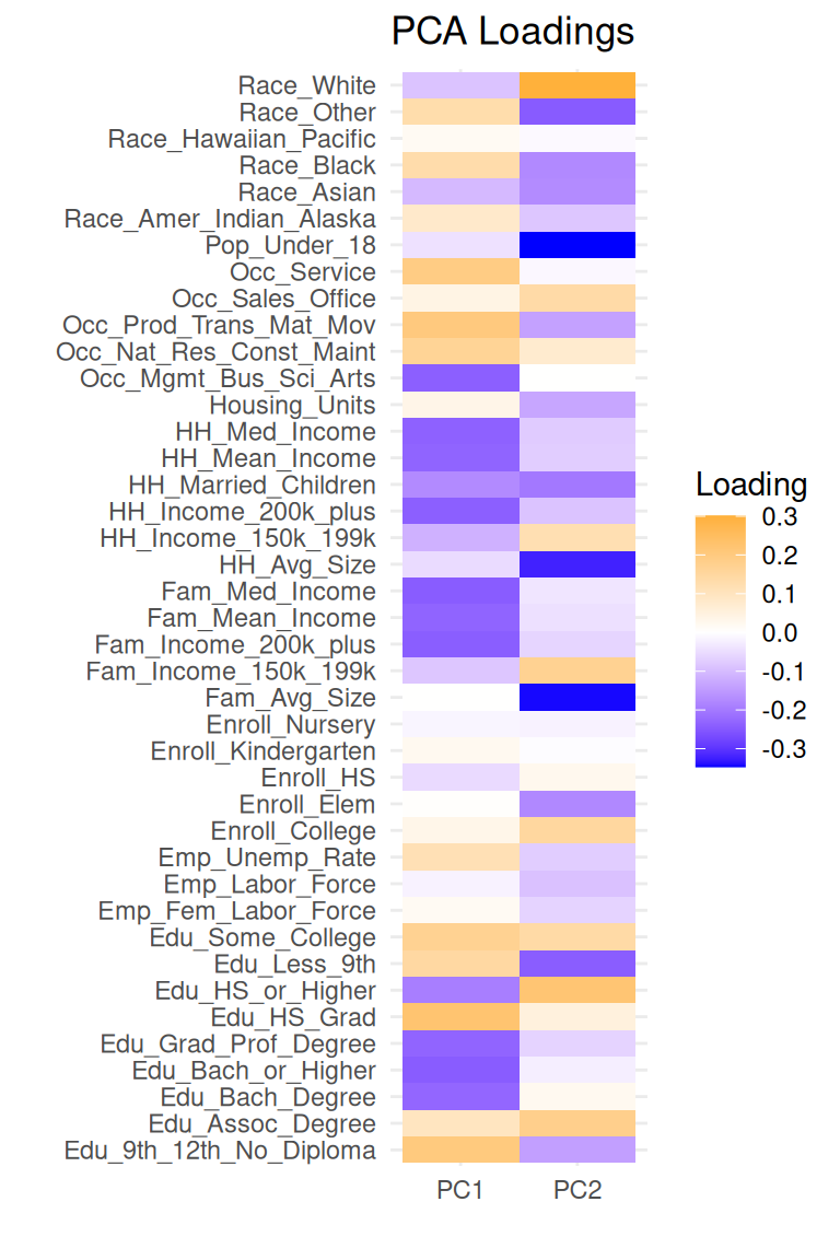
Another strategy for identifying peer districts is a dimensionality reduction technique called Principal Components Analysis. This is actually the same technique used to develop the original District Factor Groups. Though here I am using more data and more recent data. The central idea is to reduce our 40-dimensional (40-column) data set into a smaller set of components (or dimensions) that are maximally different from each other and uncorrelated with each other. These new components would contain the essence of the larger set of columns. As in the DFG calculation, I expect the first principal component to contain the variance associated with socioeconomic status (SES).
The general procedure is to:
Compute the principal components on the data set
Assess which dimensions load in which principal components
Rank order component of interest, and find districts surrounding Fair Haven
If the first one or two components is not sufficient, we are in clustering territory, which will be addressed later.
Code - Using Principal Components
# Perform PCApcadat <-na.omit(edge_df[,-c(1:3)])rownames(pcadat) <-make.unique(na.omit(edge_df)$Geography)pca_result <-prcomp(pcadat, scale.=T, center = T)#round(pca_result$sdev^2/sum(pca_result$sdev^2), 2) #first two ~49% variance, 37+12# Extract principal componentspc_all_scores <- pca_result$x#Visualize the reduced data#autoplot(pca_result, data = pcadat, label = TRUE, label.size = 3)# Get loadingspca_loadings <- pca_result$rotation# Transform loadings into a long format data frameloadings_df <-as.data.frame(pca_loadings)loadings_df$Variable <-rownames(pca_loadings)loadings_long <- reshape2::melt(loadings_df, id.vars ="Variable", variable.name ="PC", value.name ="Loading")
In Figure 1, it is clear that Component 1 (PC1) is loading on income and education dimensions, which are qualitatively aligned with SES. However, Component 2 (PC2) is loading on other potentially relevant dimensions, such as family size and the population under 18. Note the differences below in the districts that surround Fair Haven for both PC1 and PC2.
# Create heatmapggplot(loadings_long %>%filter(PC %in%c("PC1", "PC2")), aes(x = PC, y = Variable, fill = Loading)) +geom_tile() +scale_fill_gradient2(low ="blue", mid ="white", high ="orange") +theme_minimal() +labs(title ="PCA Loadings", x="", y="")
Figure 1: Loadings from first two components of the PCA.
Clustering
A final approach to identifying peer districts is cluster analysis. Cluster analysis leverages distance functions to separate districts based on similarity, with the goal of creating groups of high similarity within clusters and high dissimilarity between clusters. I will explore both K-means and hierarchical clustering techniques, looking at a few examples of each.
K-means clusters
K-means clustering requires a distance matrix as input, and I have already created Euclidean and Mahalanobis distance matrices. I can also apply distance calculations to the PCA results in order to generate clusters based on the reduced dimensionality provided by principal components. Both scaled and un-scaled PCA results are clustered. The un-scaled version should over-weight PC1, and the scaled version should treat PC1 and PC2 more equally. The tabs below show the resulting peer groups from a standard K-means routine that assumes 7 clusters (a full treatment of K-means that searches for the optimal number of clusters is omitted in this document). Each tab includes a list of districts that were clustered alongside Fair Haven given the particular distance matrix as input.
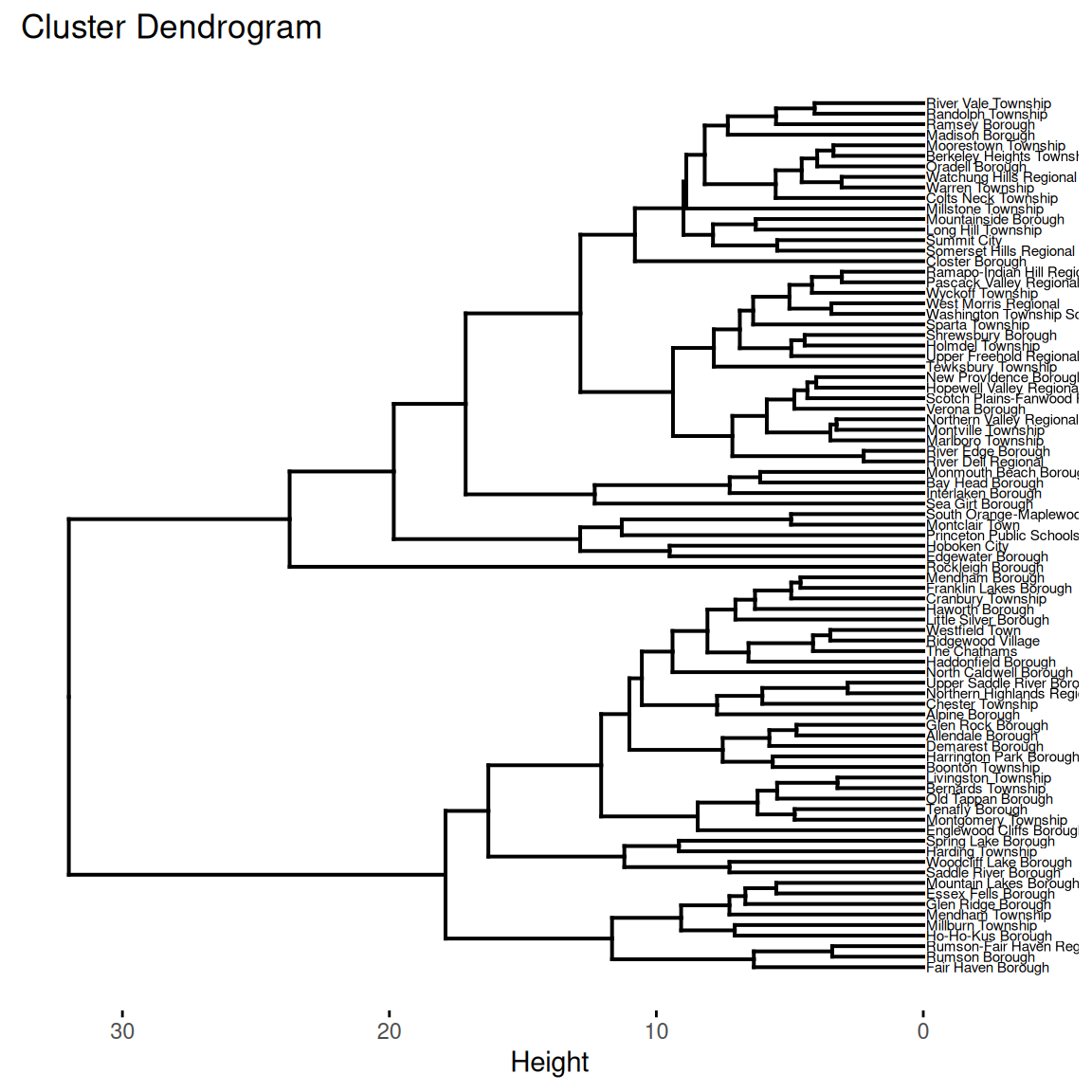
Another clustering strategy is called Hierarchical Clustering, which generates a full tree of districts based on similarity. One advantage of this technique is that one does not have to determine a priori how many clusters there are in the data. The tree can be cut at any level in order to find clusters of appropriate size.
As with K-means, the input to the hierarchical clustering routine is a distance matrix. There is another parameter included in the model to instruct how the clustering algorithm should combine districts with each other and with groups. This is often called the “method”, and here will explore a few methods. Again as with K-means, a full treatment of cluster analysis is not provided here. Rather, this exercise is to generate candidate sets of peers that will be qualitatively assessed in the next section.
The first tab below shows a partial dendrogram highlighting part of the full tree that contains a decent-sized cluster around Fair Haven. The other two tabs show the resulting peer groups from different clustering inputs.
Code - Hierarchical clustering
find_min_cluster <-function(hc, target_observation ="Fair Haven Borough", min_size =50, verbose=FALSE) {# Function to find where to cut tree to generate smallest cluster with FH that has at least 50 districts n <-length(hc$labels) min_k <-NULL min_cluster_size <-Inffor (k in2:n) { clusters <-cutree(hc, k = k) target_cluster <- clusters[names(clusters) == target_observation] cluster_members <-names(clusters[clusters == target_cluster]) cluster_size <-length(cluster_members)if (cluster_size >= min_size && cluster_size < min_cluster_size) { min_k <- k min_cluster_size <- cluster_size } } final_clusters <-cutree(hc, k = min_k)if (!is.null(final_clusters)) {# Check the size of the cluster that "Fair Haven Borough" belongs to. target_cluster <- final_clusters[names(final_clusters) == target_observation] cluster_members <-names(final_clusters[final_clusters == target_cluster]) # contains peersif (verbose) {print(paste("Size of cluster containing Fair Haven Borough:", length(cluster_members)))print(paste("Number of Clusters:", length(unique(final_clusters)))) } } else {if (verbose) print("No cluster found with size >= 50 containing Fair Haven Borough.") }if (!is.null(min_k)) {return(list(final_clusters=final_clusters, target_cluster=target_cluster, cluster_members=cluster_members)) } else {return(NULL) }}# Distance matrices:# pc_dist_scaled# pc_dist_unscaled# edge_dist# dist_mat_mah (SKIP_)# Hierarchical clustering using Ward and WPGMA Linkage## Euclideanhc_euclid_ward <-hclust(edge_dist, method ="ward.D2" )hc_euclid_mcquitty <-hclust(edge_dist, method="mcquitty")hc_euclid_ward_clusters <-find_min_cluster(hc_euclid_ward, min_size =50, target_observation = fh_leaid)hc_euclid_mcquitty_clusters <-find_min_cluster(hc_euclid_mcquitty, min_size =50, target_observation = fh_leaid)## PC scaledhc_pc_dist_scaled_ward <-hclust(pc_dist_scaled, method ="ward.D2" )hc_pc_dist_scaled_mcquitty <-hclust(pc_dist_scaled, method="mcquitty")hc_pc_dist_scaled_ward_clusters <-find_min_cluster(hc_pc_dist_scaled_ward, min_size =50, target_observation ="Fair Haven Borough School District, NJ")hc_pc_dist_scaled_mcquitty_clusters <-find_min_cluster(hc_pc_dist_scaled_mcquitty, min_size =50, target_observation ="Fair Haven Borough School District, NJ")## PC unscaledhc_pc_dist_unscaled_ward <-hclust(pc_dist_unscaled, method ="ward.D2" )hc_pc_dist_unscaled_mcquitty <-hclust(pc_dist_unscaled, method="mcquitty")hc_pc_dist_unscaled_ward_clusters <-find_min_cluster(hc_pc_dist_unscaled_ward, min_size =50, target_observation ="Fair Haven Borough School District, NJ")hc_pc_dist_unscaled_mcquitty_clusters <-find_min_cluster(hc_pc_dist_unscaled_mcquitty, min_size =40, target_observation ="Fair Haven Borough School District, NJ")
Thus far, I have created a number of candidate peer groups for Fair Haven. In fact, there are 14 possible sets to choose from (probably too many!):
Distance-based (pick districts closest to Fair Haven according to a distance metric)
Euclidean euclid_score
Mahalanobis mah_score
Principal Components (pick districts according to similarity across a reduced dimensional space)
PC1 PC1
PC2 PC2
K-means Clusters (pick districts based on groups derived from the K-means algorithm.
Euclidean distance km_euclid
Mahalanobis distance km_maha
First two principal components (scaled) km_pc_scaled
First two principal components (unscaled) km_pc_unscaled
Hierarchical Clusters
Euclidean - Ward hc_euclid_ward
Euclidean - WPGMA hc_euclid_mcquitty
PC Scaled - Ward hc_pc_dist_scaled_ward
PC Scaled - WPGMA hc_pc_dist_scaled_mcquitty
PC Unscaled - Ward hc_pc_dist_unscaled_ward
PC Unscaled - WPGMA hc_pc_dist_unscaled_mcquitty
The table below summarizes a selection of district characteristics for the districts that are included in each potential peer set (restricted to PK/K-8th grade). Fair Haven itself is included in the last row for comparison. The Peninsula column is TRUE if FH, Rumson, Little Silver, and Shrewsbury (Peninsula Peers) are all included in that particular peer set.
Group Characteristics for Districts in each Peer Set
Data from ACS-EDGE 2018-22.
Actually selecting which peer set to use at this point is a combination of art and science. I would like enough districts in the set to provide sufficient variation, but not too many to make comparisons unwieldy - between 35 and 45 should work. Ideally the “Peninsula” peers are already in the set; otherwise I would manually add them in after. It seems like the Hierarchical (Euclidean Ward) set might offer good coverage. A list of these peers can be found above at Section 4.1.4.2, and upon inspection, they do seem reasonable. The group of peers has about 72% of the population with a Bachelor’s degree or higher (FH’s 79%), median household income of $192k (FH’s $230k), and 64% of the population working in management, business, science, or arts (FH’s 60%). From the table, one could argue that that are smaller peer sets that have districts more similar to FH, but I will proceed with the hierarchical cluster-generated solution.
This concludes the section on peer set generation for Fair Haven.
Financial Data (User Friendly Budgets)
In order to understand factors related to school district financing, a data source for financial data is required. The state of New Jersey’s Department of Education provides User Friendly Budgets, which contain district-level expenses and appropriations. I mostly rely on per-pupil costs, and save them as a CSV file for easy access.
Student outcomes data come from the NJ School Performance Reports. To gather longitudinal data, I ingest report card data from 2014-15 to 2023-24. The content and format of the report cards varies greatly from year to year. I makea best effort approach to join appropriately across years.
Though there are times when it will be useful for individual data sets to be used alone, it is also useful to have one dataset that contains the latest data available, which is the 2023-24 school year as of this writing.